Examples
 Updated 3 months ago
by
Stephanie Krenz
Updated 3 months ago
by
Stephanie Krenz
Of course, we can get to our data in a shorter way in both examples. However, we have 'extended' the whole exercise a little for a clearer introduction.
The interfaces and colours have been adapted in more recent versions. The images in the screenshots may therefore differ slightly.
In the following sections, we will take a practical look at this using examples.
Example 1: simple Package
What data would we like to know or extract?
- Extraction of all positions already posted
- Of all productive Company Codes
What do we need for this extraction or where do we get this data from?
- Table with Company Codes
- Table with already posted positions from the FI-Dictionary
- Filter on the indicator whether Company Code is productive
Let's start with the integration of T001 (SAP table of Company Codes) as a table. Then we toggle all fields.
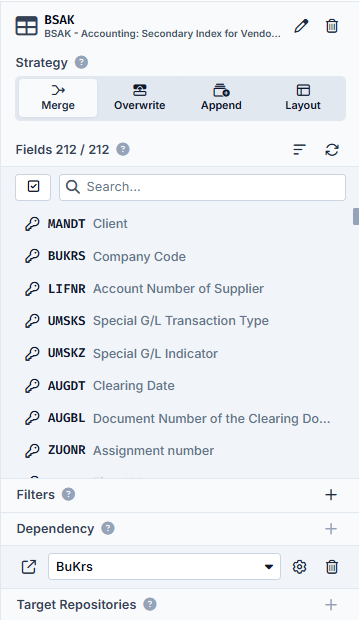
We also use the BSAK table to extract the balanced items; this is also included as a table.
Since we only want the Company Codes that are already in productive use, we create a filter -> for this example we call the filter Is_Prod.
Finally, we create a repository in which these Company Codes are saved after the first step (extraction of all productive Company Codes) in order to be able to carry out the next extraction -> in this example we call the repository BuKrs (the German equivalent of CCode).
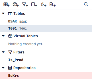
After these steps, we have the following elements on the left:
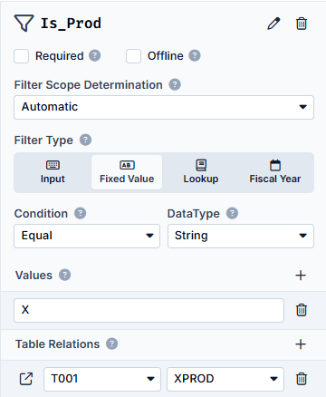
In the next step, we set the filter. As we specify in this filter that the XPROD field in the T001 must be active, i.e. must contain the value X, we enter the Type Fixed Value. As this is a character, the DataType is String and the Condition is Equal, as we are looking for exactly the value X.
We now enter the value X and in the table relations we specify that this filter is set in table T001 for the XPROD field. The Detail Area in the right-hand area now looks as follows (when selecting the filter on the left):
We now filter all entries from table T001 whose Company Codes are active (XPROD = X). We need to store this data temporarily for further use. We do this in the BuKrs repository.
We insert into the repository which fields it should contain, where these contents come from and for which other tables these values are used.
Therefore, we first insert a CCode field - if we would call this field BUKRS, the auto-mapping would take effect for the source and target tables. In this example, however, we will do this manually first.
We then specify that the source table is T001 - this is where our data comes from, which we store in this repository.
Last but not least, we specify that the BSAK table is the target table. The values from this repository will continue to be used in this table.
You will see a ⚙️ next to the respective table names on the right. This ⚙️ stands for Custom Mapping, which means that you have to link the field from the respective table with the field from the repository.
In the end, the detailed view of the repository looks like this:
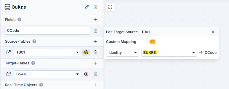
Clicking on ⚙️ opens a window with the option of linking the values in the Identity area.
Let's now take a look at the detail area of tables T001 and BSAK:
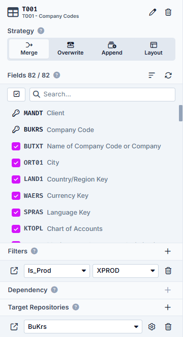
Here for T001 you can see the selected fields, the first two are the Primary Keys and the third is the indicator for whether the Company Code is used productively. The filter targets the XPROD field and the filtered Company Codes end up in the Target Repository BuKrs.
The situation is somewhat different in the detailed area of the BSAK:
Here, the data is filtered depending on the dependency of the data from the BuKrs repository.
At the end, the Element Overview in the middle looks like this:
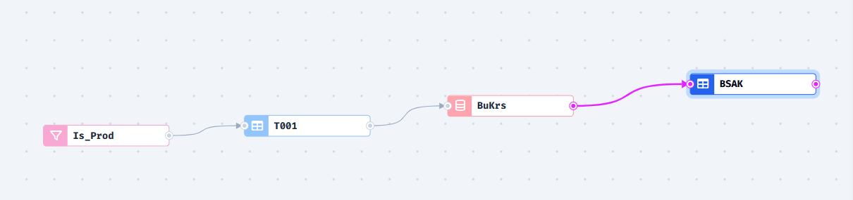
The short explanation here is:
The Is_Prod filter filters the entries from the T001. These filtered entries end up in the BuKrs repository, which is used to filter the entries from the BSAK.
At the end, you will receive a list of the posted positions from the BSAK that are assigned to a productive Company Code.
Example 2: advanced Package
What data would we like to know or extract?
- Search for all Purchase Orders (PO) from the EKKO table
- By extracting all POs with open or already paid invoice documents
- From one or more Fiscal Year(s)
- From German vendors
What do we need for this extraction or where do we get this data from?
- Tables:
- Vendor Master Data
- Accounting: Secondary Index for Vendors (Cleared Items)
- Accounting: Secondary Index for Vendors data (Open Items)
- Accounting Document Segment
- Purchasing Document Header
- Filters:
- Vendors from Germany
- Fiscal Year
- Repositories (we add them during the creation of the Package):
- ...
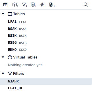
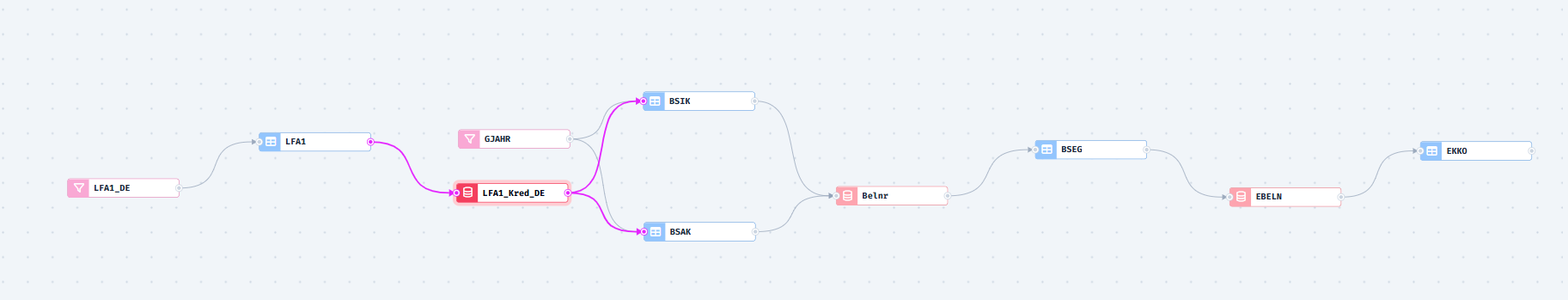
For now, let's find all the tables we need. We need:
- LFA1: Vendor Master Data
- BSAK: Accounting - Secondary Index for Vendors (Cleared Items)
- BSIK: Accounting - Secondary Index for Vendors data (Open Items)
- BSEG: Accounting Document Segment
- EKKO: Purchasing Document Header
Next, we will again create the filters and name them accordingly:
- LFA1_DE (German Vendors)
- GJAHR (Fiscal Year)
The left-hand area then looks like this:
Let's now set the filter LFA1_DE and specify which tables and fields we want to filter on:
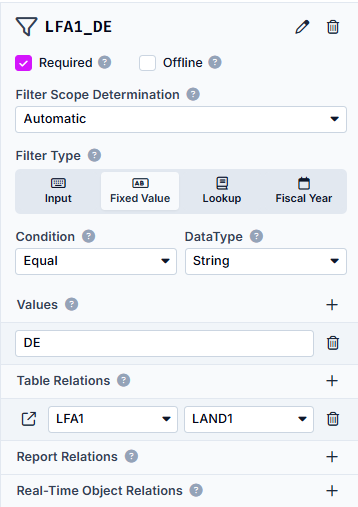
Type: Fixed Value, as we are only looking for vendors from one country and this country does not change
DataType: String, as the value is a character string
Condition: Equal, as this value is fixed and cannot vary
Values: DE, Country Key for Germany
Table Relations: LFA1 with the field LAND1, Table and Field, on which the filter is set
Now the second filter:
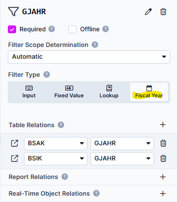
Type: Fiscal Year
Condition: Equal, as we only search for the Fiscal Years that are entered as parameters later in the task
Table Relations: BSAK and BSIK, both with the field GJAHR
Now that we have successfully created the tables and filters, let's turn our attention to the repositories that are needed to save the intermediate results with which we can then continue working.
In this example, we have set the field name in the repository to the same as the field name in the tables. You can see the effect of this in the next section.
In the first step, we filter the table LFA1 with the filter LFA1_DE. We create the repository LFA1_Kred_DE to store these results temporarily.
We define the following settings for this repository:
- Fields
- LIFNR: for storing the Vendor Numbers of the German suppliers
- Target-Tables
- BSIK: same automatic assignment of the fields via the LIFNR
- BSAK: same automatic assignment of the fields via the LIFNR
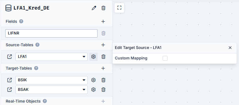
We now have our first repository that contains all Vendor Numbers of German suppliers.
In the next step, we want to filter the BSAK and BSIK tables: we want the document numbers as a result, filtered on the one hand with the Vendor Numbers just found and on the other hand with the Fiscal Year(s) entered in the task.
To do this, we create another repository with the document numbers found here and call it Belnr.
But now we have to be careful: Saving only the document numbers here would mean that we would either not receive all document numbers or have numerous duplicate entries. This is because the document number can be repeated in the Company Codes and the Fiscal Years. To counteract this, we therefore not only include the document number in the Repository, but also the Fiscal Year and the Company Code.
As this information comes from the BSAK and BSIK Tables, we specify these two as Source Tables.
And now our second repository is ready:
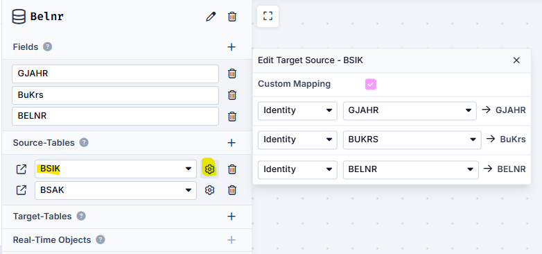
We now have the document numbers of German vendors from the desired Fiscal Year(s) in our repository Belnr.
Now we look for the POs from the BSEG table.
This means that the BSEG is filtered as a Dependency of our Repository Belnr.
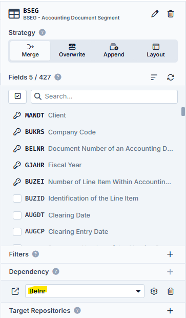
Due to the different spelling of the field for the Company Code, the Custom Mapping must also be carried out here again.
We now write the data obtained here to the next and final repository, which we call EBELN.
As the PO numbers are unique in our example, we only need one field here, which is also called EBELN. We specify that the data stored here comes from the BSEG table (therefore as a source table).
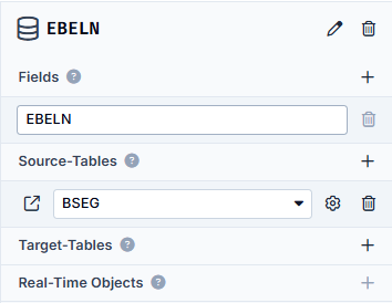
And since we have now paid attention to the correct spelling of upper and lower case, the automatic mapping takes effect again.
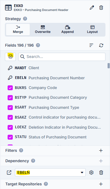
At the end, we want to filter the EKKO table with the POs found in order to obtain all other order header information. We now include the EKKO. As we want to extract all available information here, we now select all fields with the All button. This table is filtered again depending on the Dependency of the previous Repository EBELN.
And et voilà! In the end, we have all the relevant order header data from the desired Fiscal Year(s) from German vendors.
Finally, if we look at the Element Overview in the middle, the whole thing looks like this:
The following results tables are currently displayed:
- LFA1
- BSAK & BSIK
- BSEG
- EKKO
If you are really only interested in the order header data, you can also change the LFA1, BSAK & BSIK and BSEG tables to Virtual Tables. These are then no longer saved as result tables at the end.